Chapter 7 Analysis covariates

Once we have created the building blocks for our data analysis dataframes, we must bring in the variables which will be used in the modelling steps. It is important to not that there are millions of ways to add covariates - both in terms of how you do it, and where you derive the data from. The covariates you use will depend on the questions you have, and the context of your survey. The examples provided here are not comprehensive and serve only as a guide!

Create a new .R script

Call it 02_example_covariates.R.

Load the required packages

library(kableExtra);library(dplyr); library(sf); library(modisfast); library(lubridate); library(corrplot); library(traitdata); library(terra); library(osmdata); library(elevatr)

We can simplify the covariate options we have available into two distinct categories:

- Species traits

The traits are species-level covariates which we think are important in structuring their responses to other covariates, such as human modification.

# Start by reading in your species list
sp_summary <- read.csv("data/processed_data/AlgarRestorationProject_species_list.csv", header=T)

- Location-level covariates

Location-level covariates are characteristics of the camera locations which are either fundamental to your question (such as the habitat type, degree of human modification, or distance to the nearest road), or they are things you are not directly interested in but must account for in your analyses. The way we derive and treat these variables are identical however.

locs <- read.csv("data/processed_data/AlgarRestorationProject_camera_locations.csv", header=T)

7.1 Species traits

It is easier than ever before to add trait data to your species lists, particularly with the advent of R packages which pool multiple data sources such as the traitdata database, which to date, compiles data from 32 different sources.

Below we use this package to add trait data to the project species list:

# This package isn't available on Cran, so we must use the remotes package
#library(remotes)
#remotes::install_github("RS-eco/traitdata", build_vignettes = T, force=T)
# Load the library
library(traitdata)

To pull the data for a specific database we use the following code:

data("elton_mammals")

To explore the full list of available datasets click this link.

Let’s take a look at what categories we have available to us:

 head(elton_mammals) %>% kbl() %>% scroll_box(height = "200px") %>%
  kable_paper("striped", full_width = F)

MSW3_ID	Genus	Species	Family	Diet.Inv	Diet.Vend	Diet.Vect	Diet.Vfish	Diet.Vunk	Diet.Scav	Diet.Fruit	Diet.Nect	Diet.Seed	Diet.PlantO	Diet.Source	Diet.Certainty	ForStrat.Value	ForStrat.Certainty	ForStrat.Comment	Activity.Nocturnal	Activity.Crepuscular	Activity.Diurnal	Activity.Source	Activity.Certainty	BodyMass.Value	BodyMass.Source	BodyMass.SpecLevel	Full.Reference	scientificNameStd
1	Tachyglossus	aculeatus	Tachyglossidae	100	0	0	0	0	0	0	0	0	0	Ref_1	ABC	G	A		1	1	0	Ref_1	ABC	3025.00	Ref_117	1	Nowak R.M. (1999). Walker’s mammals of the world. Sixth edition edn. The Johns Hopkins University Press, Baltimore, Maryland	Tachyglossus aculeatus
2	Zaglossus	attenboroughi	Tachyglossidae	100	0	0	0	0	0	0	0	0	0	Ref_65	ABC	G	A		1	0	0	Ref_1	ABC	8532.39	Ref_2, Ref_3	0	Leary, T., Seri, L., Flannery, T., Wright, D., Hamilton, S., Helgen, K., Singadan, R., Menzies, J., Allison, A., James, R., Aplin, K., Salas, L. & Dickman, C. 2008.�Zaglossus attenboroughi. In: IUCN 2010. IUCN Red List of Threatened Species. Version 2010.	Zaglossus attenboroughi
3	Zaglossus	bartoni	Tachyglossidae	100	0	0	0	0	0	0	0	0	0	Ref_2	D1	G	A		1	0	0	Ref_1	ABC	7180.00	Ref_131	1	Genus Average	Zaglossus bartoni
4	Zaglossus	bruijni	Tachyglossidae	100	0	0	0	0	0	0	0	0	0	Ref_1	ABC	G	A		1	0	0	Ref_1	ABC	10139.50	Ref_117	1	Nowak R.M. (1999). Walker’s mammals of the world. Sixth edition edn. The Johns Hopkins University Press, Baltimore, Maryland	Zaglossus bruijni
5	Ornithorhynchus	anatinus	Ornithorhynchidae	80	0	0	20	0	0	0	0	0	0	Ref_1	ABC	G	A		1	1	1	Ref_1	ABC	1484.25	Ref_117	1	Nowak R.M. (1999). Walker’s mammals of the world. Sixth edition edn. The Johns Hopkins University Press, Baltimore, Maryland	Ornithorhynchus anatinus
6	Caluromys	philander	Didelphidae	20	0	0	0	10	0	20	0	10	40	Ref_1	ABC	Ar	A		1	1	0	Ref_1	ABC	229.25	Ref_117	1	Nowak R.M. (1999). Walker’s mammals of the world. Sixth edition edn. The Johns Hopkins University Press, Baltimore, Maryland	Caluromys philander

Lets make a new column sp which matches the species column in our ‘sp_summary’ dataset. We will use this as the “key” variable to extract the trait data.

elton_mammals$sp <- paste0(elton_mammals$Genus,"." ,elton_mammals$Species)

We do not want to take all of the trait data, so lets subset to BodyMass.Value and the activity data Activity.Nocturnal Activity.Crepuscular Activity.Diurnal.

tmp <- elton_mammals[, c("sp","BodyMass.Value", "Activity.Nocturnal", "Activity.Crepuscular",   "Activity.Diurnal")]

# Lets rename the columns to make them more usable
tmp <- tmp %>% rename(
              mass_g = BodyMass.Value,
              act_noct = Activity.Nocturnal,
              act_crep = Activity.Crepuscular,
              act_diur = Activity.Diurnal)

sp_summary <- left_join(sp_summary, tmp)

And then check our output:

sp_summary %>% kbl() %>% scroll_box(height = "200px") %>%
  kable_paper("striped", full_width = F)

class	order	family	genus	species	sp	common_name	mass_g	act_noct	act_crep	act_diur
Mammalia	Artiodactyla	Cervidae	Alces	alces	Alces.alces	moose	356998.16	1	1	0
Mammalia	Artiodactyla	Cervidae	Cervus	canadensis	Cervus.canadensis	elk	NA	NA	NA	NA
Mammalia	Artiodactyla	Cervidae	Odocoileus	virginianus	Odocoileus.virginianus	white-tailed deer	55508.56	1	1	0
Mammalia	Artiodactyla	Cervidae	Rangifer	tarandus	Rangifer.tarandus	caribou	86033.98	0	0	1
Mammalia	Carnivora	Canidae	Canis	latrans	Canis.latrans	coyote	13406.33	1	1	0
Mammalia	Carnivora	Canidae	Canis	lupus	Canis.lupus	gray wolf	32183.33	1	1	0
Mammalia	Carnivora	Canidae	Vulpes	vulpes	Vulpes.vulpes	red fox	5476.17	1	1	0
Mammalia	Carnivora	Felidae	Lynx	canadensis	Lynx.canadensis	canada lynx	9373.25	1	0	0
Mammalia	Carnivora	Mustelidae	Lontra	canadensis	Lontra.canadensis	river otter	8087.42	1	1	0
Mammalia	Carnivora	Mustelidae	Martes	americana	Martes.americana	american marten	1250.00	1	0	0
Mammalia	Carnivora	Ursidae	Ursus	americanus	Ursus.americanus	black bear	99949.36	1	0	0
Mammalia	Lagomorpha	Leporidae	Lepus	americanus	Lepus.americanus	snowshoe hare	1710.02	1	0	0
Mammalia	Lagomorpha	Leporidae	Oryctolagus	cuniculus	Oryctolagus.cuniculus	rabbit	1832.22	1	0	0
Mammalia	Rodentia	Sciuridae	Tamiasciurus	hudsonicus	Tamiasciurus.hudsonicus	red squirrel	201.17	0	0	1

If there are any NA’s, it could be for several reasons:

1. There is no trait data for that species - in this case you could either:

• leave them as NA’s (excluding them from later analyses) or if you are lucky, your analysis framework might be able to accommodate missing trait data

• Give the species the mean values obtained from other species in its genus

2. There is a mismatch in taxonomic resolution - you are working with a subspecies that isn’t recognized. This is the case here with elk! Lets replace it with the data for (Cervus elaphus)

sp_summary[sp_summary$sp=="Cervus.canadensis", c("mass_g", "act_noct","act_crep","act_diur")] <- 
    elton_mammals[elton_mammals$sp=="Cervus.elaphus", c("BodyMass.Value", "Activity.Nocturnal", "Activity.Crepuscular", "Activity.Diurnal")]

Whatever you do, remember to report it in your methods section!

Let’s save our species list for a rainy day!

write.csv(sp_summary, paste0("data/processed_data/", locs$project_id[1],"_species_list.csv"), row.names = F)

7.2 Camera station covariates

It is common to have a suite of covariates which you would like to investigate the effects of in your datasets. These could take the form of habitat designations or treatment types. These may already be included with your deployment data, or you may need to derive them from a variety of remote sources. In their simplest form, these variable are time invariant (they do not change), however you may have variables which change through time as well (we discuss these at the end). In the following steps, we walk through the process of manipulating and deriving example covariates.

For the time invariant covariates, we will add them to our locs dataframe imported above.

7.2.1 Locally collected covariates

You may have collected some data in the field when deploying or checking your camera traps, and kept that data separate from your camera trap data (e.g. vegetation assessments). Provided that the naming convention you gave to these dataframes is the same as in your camera data (e.g. the location is in a column called placename) - you can do a ’left_join()` to merge the two datasets.

Import a sample set of local covariates:

local_covs <- read.csv("data/raw_data/example_covariates/example_dataframe.csv")

Lets take a look at the data structure:

placename	line_of_sight_m
ALG001	137.12500
ALG002	131.52778
ALG003	353.65833
ALG004	158.04167
ALG005	305.81944
ALG006	60.12500
ALG007	310.58333
ALG008	112.75000
ALG009	299.02778
ALG010	102.30556
ALG011	223.56944
ALG012	140.91667
ALG013	394.56944
ALG014	196.87500
ALG015	163.11111
ALG016	116.11111
ALG017	138.19444
ALG018	304.29167
ALG019	330.97222
ALG020	204.40278
ALG021	264.94444
ALG022	229.13889
ALG023	218.29167
ALG024	425.43056
ALG025	56.97222
ALG026	200.05556
ALG027	252.95833
ALG028	277.50000
ALG029	206.52778
ALG030	43.38889
ALG031	334.27778
ALG032	83.00000
ALG033	165.00000
ALG034	337.79167
ALG035	439.61111
ALG036	62.69444
ALG037	392.61111
ALG038	352.75000
ALG039	339.76389
ALG040	182.75000
ALG041	109.25000
ALG042	219.56944
ALG043	62.41667
ALG044	374.26389
ALG045	294.83333
ALG046	34.50000
ALG047	363.80556
ALG048	392.93056
ALG049	80.77778
ALG050	139.36111
ALG051	208.12500
ALG052	13.95833
ALG053	99.30556
ALG054	35.47222
ALG055	189.06944
ALG056	55.41667
ALG057	93.04167
ALG058	80.91667
ALG059	41.00000
ALG060	189.90278
ALG061	11.16667
ALG062	16.00000
ALG063	28.94444
ALG064	34.27778
ALG065	20.11111
ALG066	36.94444
ALG067	188.83333
ALG068	72.27778
ALG069	22.85556
ALG070	28.61111
ALG071	20.05556
ALG072	52.44444
ALG073	55.94444

It is a dataframe where the survey locations are rows and the local covariates, in this case line_of_sight_m, are columns.

To add this data to our station data, we use a left_join() operation from the dplyr() package. It uses a key variable which is common in both data frames to add data from the “right-hand side” to the rows in the “left-hand side” which are not already present. Any rows present in the right-hand side which are not in the left-hand side will be skipped.

locs <- left_join(locs, local_covs)   # From the dplyr package

For more examples of joins using dplyr() see: https://dplyr.tidyverse.org/reference/mutate-joins.html

7.2.2 Remotely collected covariates

To exploit remotely collected data sources we need to use a package to help us with spatial data.

7.2.2.1 Key skills: sf package

The most intuitive package to learn spatial operations in R is the simple features package (a.k.a. sf). sf allows you to use spatial dataframes in the style of a typical R dataframe. We use this package frequently as it allows you to rapidly change coordinate projection systems (e.g. lat/long to UTM) and rapidly perform spatial operations.

Lets convert our “normal” dataframe to an sf dataframe:

locs_sf <- st_as_sf(locs,                              # We specify the dataframe 
                    coords=c("longitude", "latitude"), # The XY coordinates
                    crs=4326)                          # And the projection code

What does an sf object look like? Like a normal dataframe but with a weird header:

locs_sf

## Simple feature collection with 38 features and 4 fields
## Geometry type: POINT
## Dimension:     XY
## Bounding box:  xmin: -112.6467 ymin: 56.15983 xmax: -112.3848 ymax: 56.49352
## Geodetic CRS:  WGS 84
## First 10 features:
##                 project_id placename feature_type line_of_sight_m
## 1  AlgarRestorationProject    ALG027     HumanUse       252.95833
## 2  AlgarRestorationProject    ALG029     HumanUse       206.52778
## 3  AlgarRestorationProject    ALG031     HumanUse       334.27778
## 4  AlgarRestorationProject    ALG032     HumanUse        83.00000
## 5  AlgarRestorationProject    ALG035     HumanUse       439.61111
## 6  AlgarRestorationProject    ALG036     NatRegen        62.69444
## 7  AlgarRestorationProject    ALG037     HumanUse       392.61111
## 8  AlgarRestorationProject    ALG038     HumanUse       352.75000
## 9  AlgarRestorationProject    ALG039     HumanUse       339.76389
## 10 AlgarRestorationProject    ALG043     NatRegen        62.41667
##                      geometry
## 1   POINT (-112.4735 56.3328)
## 2  POINT (-112.5483 56.39474)
## 3   POINT (-112.482 56.30899)
## 4  POINT (-112.3968 56.40197)
## 5  POINT (-112.4761 56.38428)
## 6  POINT (-112.4058 56.23178)
## 7  POINT (-112.4449 56.27898)
## 8  POINT (-112.4792 56.27039)
## 9  POINT (-112.4094 56.30127)
## 10 POINT (-112.5842 56.38715)

That header is important - it tells you the type of data you have (lines, points, polygons etc), and the projection information (CRS).

We like using sf as it is very easy to transform coordinates into different projections using st_transform(). Use the website epsg.io to find the CRS codes for the projection you want - e.g. UTM 12N = 26712, then plug it into the following:

locs_utm <- st_transform(locs_sf, crs=26712)

Check the header of locs_utm and you should see that the CRS has changed!

Plotting sf objects is a little bit odd at first. If you try to plot them normally you get lots of replicated plots (one for each column) - try it:

plot(locs_utm)

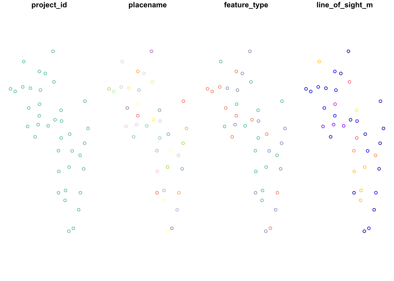
It can be useful as it varied the colors based on the properties of the column. Typically, however, we just want to plot the points themselves. We do that by wrapping the object in st_geometry() this just extracts the geometry of the object.

plot(st_geometry(locs_utm))
axis(1)
axis(2)

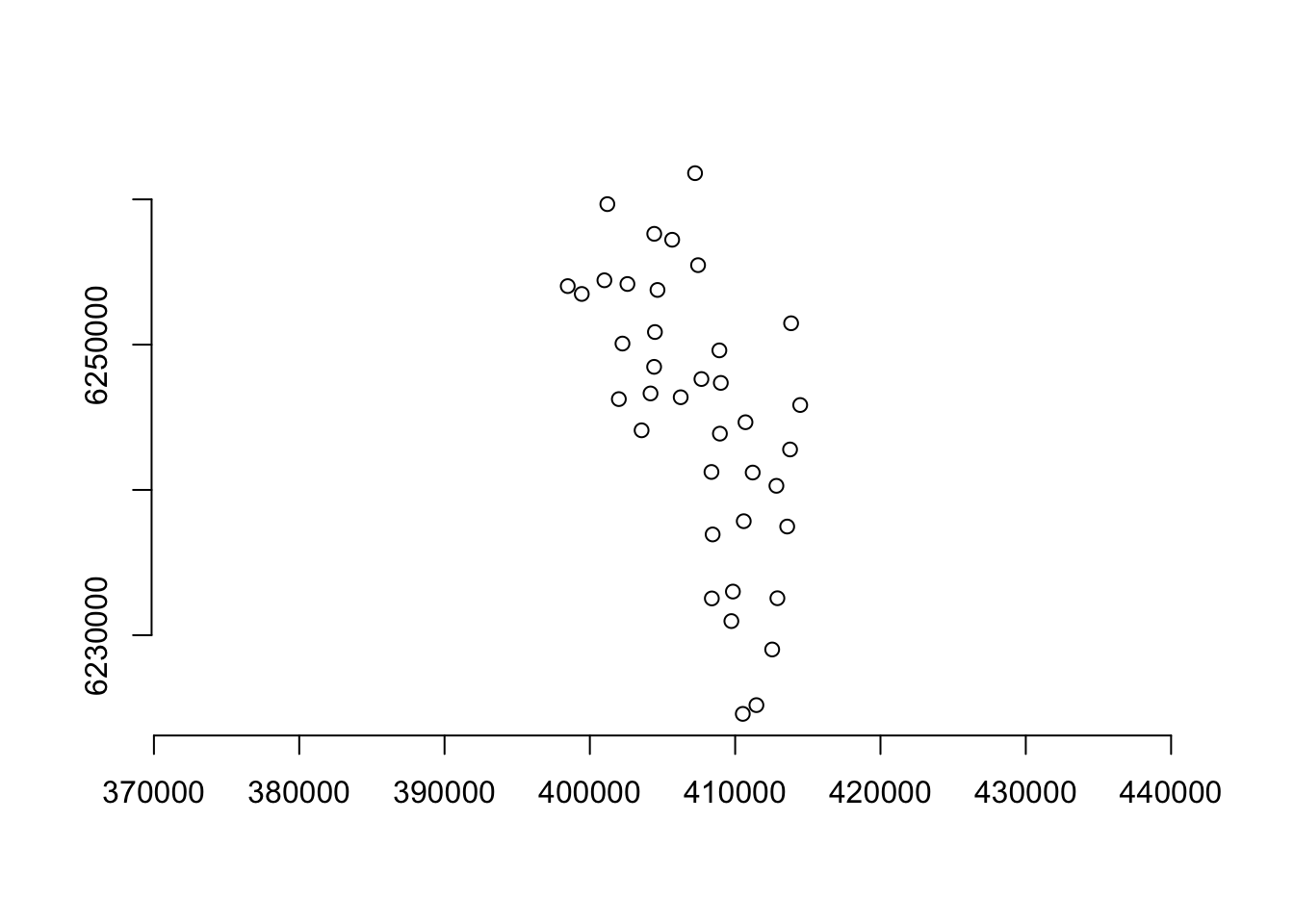
We will use st_geometry() frequently below.

For more in depth information of sf functionality see: https://r-spatial.github.io/sf/articles/sf1.html

7.2.3 Extracting data from local rasters

Often we have raster data layers stored which we would like to link to our camera locations. We have included one such example here, a raster which reflects the depth from the soil surface to the water table - a proxy for habitat type in this study site. The layer comes from the 1m Wet Area Mapping (WAM) layer:

White, Barry, et al. “Using the cartographic depth-to-water index to locate small streams and associated wet areas across landscapes.” Canadian Water Resources Journal 37.4 (2012): 333-347.

NOTE the raster has been down scaled to reduce its size for this course - it is no longer at 1m resolution.

The only time we deviate from the sf package is to deal with rasters. Raster objects in R are processed really slowly, especially if the raster is large. So instead we use the terra package.

library(terra)
# Import the example raster using the stars package
ras <- rast("data/raw_data/example_covariates/example_raster.tif")
# Covert your sf locations to the same projection as your raster then put it in terra `vect` format,
locs_terra <- locs_sf %>% 
                st_transform(crs=st_crs(ras)) %>% # change the projection to match the raster
                vect() # Turn it into a terra object

Lets check our layers match up!

plot(ras) # The terra package makes nice raster plots with legends
plot(locs_terra, add=T) # Add the survey locations as black dots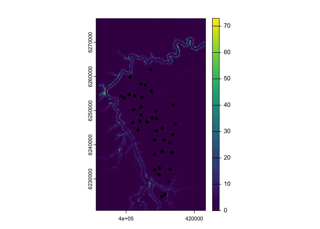

Great! Now lets buffer our camera locations by 250 meters, and take the average depth to water for each location:

# Buffer by 250m
locs_terra <- buffer(locs_terra,250)

# Extract the values to a temporary object - tmp 
tmp <- terra::extract(ras, locs_terra, fun=mean)

# Make a new column in locs_sf called water_depth_m
# They are ordered the same way so no need for a fancy join
locs_sf$water_depth_m <- tmp$Depth2WatAlgar

Finally, lets check the distribution of our data!

# Basic boxplot in base R
boxplot(locs_sf$water_depth_m)

Most locations are on the water table (lowland sites), others are above it (upload sites), and they have different vegetation characteristics in the field.

7.2.4 elevatr package

Camera studies often occur over a range of elevations - and we can quickly extract these elevations using the elevatr package and an sf dataframe.

We can extract elevation from Amazon Web Service Terrain Tiles… available globally!

locs_sf <- get_elev_point(locs_sf, 
                          src="aws", #Amazon Web Service Terrain Tiles - available globally
                          z = 12)  # z specifies the zoom level -> the lower the value the faster the code runs, but the coarser the elevation values are

## Mosaicing & Projecting

## Note: Elevation units are in meters

The src option specifies the sources of the DEM data. We use aws Amazon Web Service Terrain Tiles.

The z option specifies the resolution of the underlying DEM, the high the value, the more detailed it is. However, it will take longer to run so do not go crazy.

boxplot(locs_sf$elevation)

An elevation of ~ 500m was expected. Great!

If you want to download a full elevation raster for your area of interests, see the introduction to elevatr

7.2.5 Open Street Maps

Open Street Map (OSM) is an incredible resource for generating covariates for camera trap studies. For example, we might be interested in the distance to the nearest rivers, roads, or trails. All of these anthropogenic features are available in OSM!

CAREFUL OSM data is user contributed and often incomplete and patchy. Always plot your data and never assume it is complete without checking it first. For an example fo this see water bodies below.

First lets load the osmdata package.

library(osmdata)

The types of features we can extract using the osmdata package are listed here: https://wiki.openstreetmap.org/wiki/Map_features.

7.2.5.1 Highways

Camera trap projects are often interested in human disturbance, of which, highways are an important part.

Let’s start by defining our area of interest. All osmdata queries begin with a bounding box defining the area of the query:

# First buffer our points by 10km to create an area of interest (aoi)
aoi <- st_bbox(st_buffer(locs_sf, 10000)) # Units are in meters 

We then use this bounding box to return all of the features which cross into it:

highway <- opq(aoi) %>% #using the bounding box
           add_osm_feature(key="highway") %>% #extract all highway features
           osmdata_sf()  # convert them into simple features format

The data you extract is its own “class” of data made up from multiple data types:

str(highway)

Which looks very intimidating! However, the key thing is that it is made up of multiple data slices, each of which represents an sf dataset. Let’s take a look at three of these

• $osm_points
• $osm_lines
• $osm_polygons

par(mfrow=c(1,3))
plot(st_geometry(highway$osm_points), main="osm_points")
plot(st_geometry(highway$osm_lines), main="osm_lines")
plot(st_geometry(highway$osm_polygons), main="osm_polygons")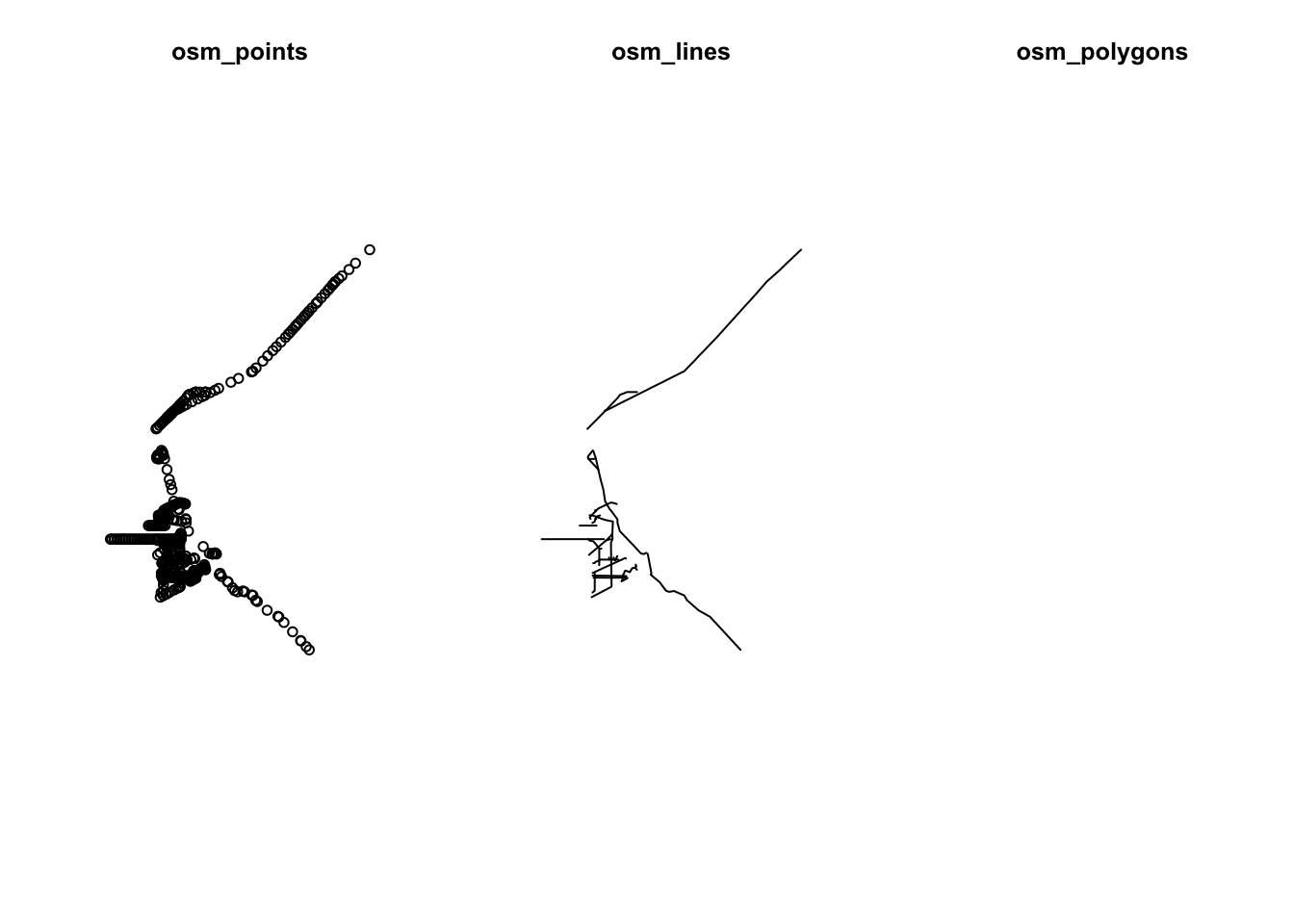

The points or the lines datasets look must useful to us, there is nothing in the polygon layer.

Let’s use the lines element and add out camera stations:

par(mfrow=c(1,1))
plot(st_as_sfc(aoi))     # st_as_sfc created a polygon from a `bbox` object
plot(st_geometry(highway$osm_lines), add=T)
plot(st_geometry(locs_sf), col="red", add=T)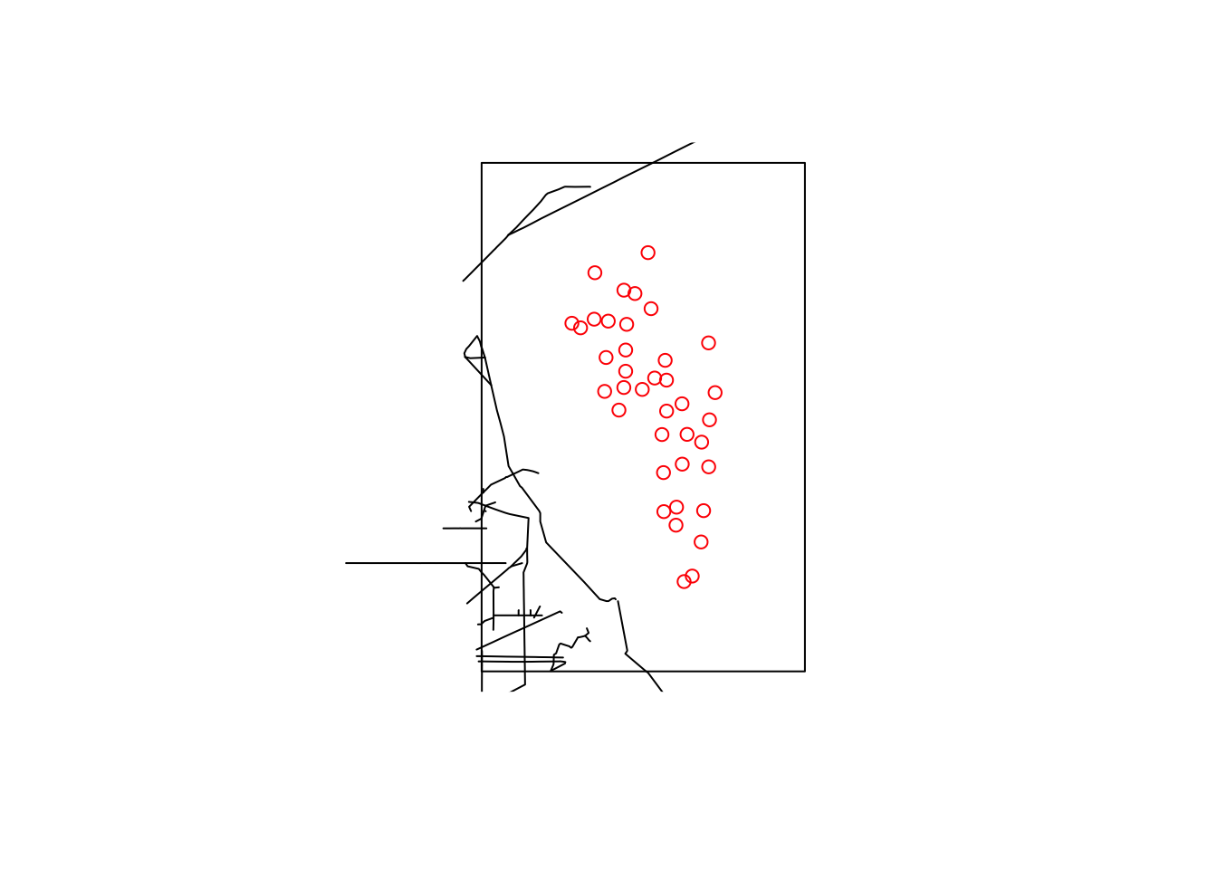

We can now calculate the distances from our cameras to these objects using the following codes:

st_nearest_feature gives us the index number of the feature which is closest to each station.

We can the use this to request the distance from that nearest feature to each camera station using st_distance. Which, put together, looks like:

# Create an index of the nearest object in `highway$osm_lines` to locs_sf
index <- st_nearest_feature(locs_sf, highway$osm_lines)

# Use that index to ask for the distance to that object
locs_sf$road_dist_m <- st_distance(locs_sf, highway$osm_lines[index,], 
                                   by_element=T) # Note `by_element=T` tells st_distance to evaluate things line by line. 

7.2.5.2 water bodies

We also might want to calculate the distances to the nearest water body, and important resource for wildlife. We can do that using the following:

water <- opq(aoi) %>%
           add_osm_feature(key = 'natural', value = 'water') %>%
           osmdata_sf()

Lets check our data:

par(mfrow=c(1,2))
plot(st_geometry(water$osm_points), main="osm_points")
#plot(st_geometry(water$osm_lines), main="osm_lines") # lines is empty and wont plot
plot(st_geometry(water$osm_polygons), main="osm_polygons")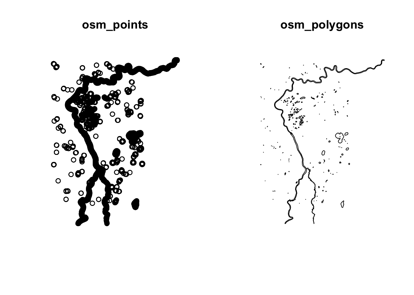

In this instance, the lines is empty, out best bet are the points or the polygons options!

index <- st_nearest_feature(locs_sf, water$osm_polygons)

locs_sf$water_dist_m <- st_distance(locs_sf, water$osm_polygons[index,], by_element=T) # Note `by_element=T` tells st_distance to evaluate things line by line. 

For more examples of using the osmdata package see: the projects github page

7.2.6 Vegetation productivity

7.2.6.1 modisfast

modisfast is an R package designed for easy and fast downloads of MODIS Land products, VIIRS Land products, and GPM (Global Precipitation Measurement Mission) Earth Observation data. It allows for easy access to time series data accross large spatial extents directly to your computer! These are the data layers commonly used to extract normalized difference vegetation index (NDVI) and Enhanced Vegetation Index (EVI) information. When using modisfast you should reference:

Taconet et al., (2024). modisfast: An R package for fast and efficient access to MODIS, VIIRS and GPM Earth Observation data. Journal of Open Source Software, 9(103), 7343,

For a quick into to the package see: https://github.com/ptaconet/modisfast

IMPORTANT to use this package you should create your own login for the Earthdata servers, then specify your EOSDIS credentials.

To create your free account go to : https://urs.earthdata.nasa.gov/.

Let’s load the package:

library(modisfast)

# Specify your own credentials:
log <- mf_login(credentials = c("your_username", "your_password")) # set your own EOSDIS username and password

For modisfast to work, we need to provide a sf polygon with an “id” column. We can do this easily using the aoi object we created earlier”

# Create aoi if sf format
aoi_sf <- st_as_sf(data.frame(id = "algar", geom = st_as_sfc(aoi), wkt = "geom", crs = 4326)) # a ROI of interest, format sf polygon

# MODIS collections and variables (bands) of interest
collection <- "MOD13Q1.061" # run mf_list_collections() for an exhaustive list of collections available
variables <- c("_250m_16_days_NDVI") # run mf_list_variables("MOD13Q1.061") for an exhaustive list of variables available for the collection "MOD13A3.061"

# Specify the time range - we will use a winter-summer transition
time_range <- as.Date(c("2019-03-01", "2019-07-01")) # a time range of interest

We then use these to specify the location of the data and download it to our computers.

## Get the URLs of the data
urls <- mf_get_url(
  collection = collection,
  variables = variables,
  roi = aoi_sf,
  time_range = time_range
)

## Download the data. By default the data is downloaded in a temporary directory, but you can specify a folder
res_dl <- mf_download_data(urls, parallel = TRUE)

# Import it into R
r <- mf_import_data(
  path = dirname(res_dl$destfile[1]),
  collection = collection,
  proj_epsg = 26912
)

Easy!

Lets see what it looks like:

# Plot the resulting NDVI data
terra::plot(r, col = rev(terrain.colors(20)), 
            range=c(0,1)) # Specify the range of values you want to plot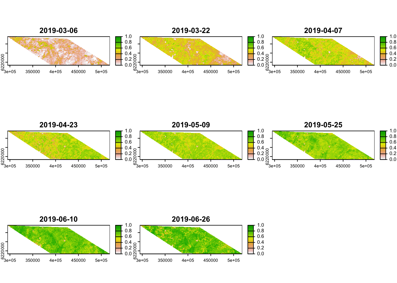

Add the data to your locations covariates dataframe and check the output:

# Extract the data to camera locations
tmp <- terra::extract(r, locs_terra, fun=mean, ID=F) # Extract - each layer will become its own column
locs_sf$mean_ndvi <- rowMeans(tmp) # take the mean of each column

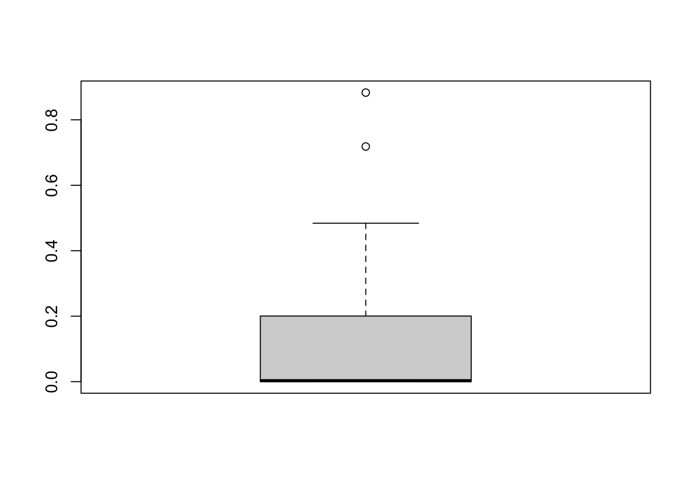
# Plot the results
boxplot(locs_sf$mean_ndvi,
        ylab="Mean NDVI score",
        las=1)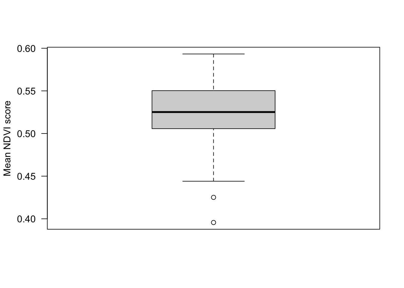

Here we have created an average NDVI score across five months, but we could get monthly averages. Some products are even available at daily resolution!

7.2.7 Digging deeper

If you want to dig into estimating NDVI metrics from camera trap viewshed, rather than from satellite data, check out the phenopix R package. It allows the user to extract visual information from time lapse images. It provides a quantitative daily measure of vegetation phenology at each site (e.g. green-up, senescence, snow cover).

Alberton, B. et al. 2017. Introducing digital cameras to monitor plant phenology in the tropics: applications for conservation. Perspect. Ecol. Conserv

Filippa, G. et al. 2017. phenopix: Process Digital Images of a Vegetation Cover. R package version 2.3.1.

The Phenopix package has a five step process:

1. a region of interest (ROI) is identified;
2. the red, green, and blue digital numbers from each image in the time series is extracted and an index of relative ‘greenness’ is computed and plotted from the digital numbers;
3. the vegetation indices’ data points are filtered to remove inconsistencies;
4. a curve is fit to the data and phenophases are determined from the curve;
5. phenophase uncertainties are calculated.

To see an application and comparison of these metrics, we highly recommend that you check out Catherine Sun’s (WildCo alumni) paper on the subject:

Sun, Catherine, et al. “Simultaneous monitoring of vegetation dynamics and wildlife activity with camera traps to assess habitat change.” Remote Sensing in Ecology and Conservation 7.4 (2021): 666-684.

And the code associated with this publication on the WildCo GitHub Page

7.3 Convert and save your covariates

# Convert columns to numeric
locs_sf$road_dist_m <- as.numeric(locs_sf$road_dist_m)

# Convert it back to a dataframe
locs_sf$geometry <- NULL

locs <- left_join(locs, locs_sf)


# Write the dataset

write.csv(locs, paste0("data/processed_data/", locs$project_id[1],"_camera_locations_and_covariates.csv"), row.names=F)

7.4 Correlations between predictors

So we have used a variety of different techniques to generate covariates for our subsequent analyses. However, it is important to note that we cannot just through these variables into a model.

One way to check if your different variables are confound/correlated is using the corrplot package.

library(corrplot)

# First we need to create a correlation matrix between the different variables of interest
M <- cor(locs[, c("line_of_sight_m", "water_depth_m", "elevation",
                     "road_dist_m", "mean_ndvi")])

Now lets make the basic corrplot:

corrplot(M)

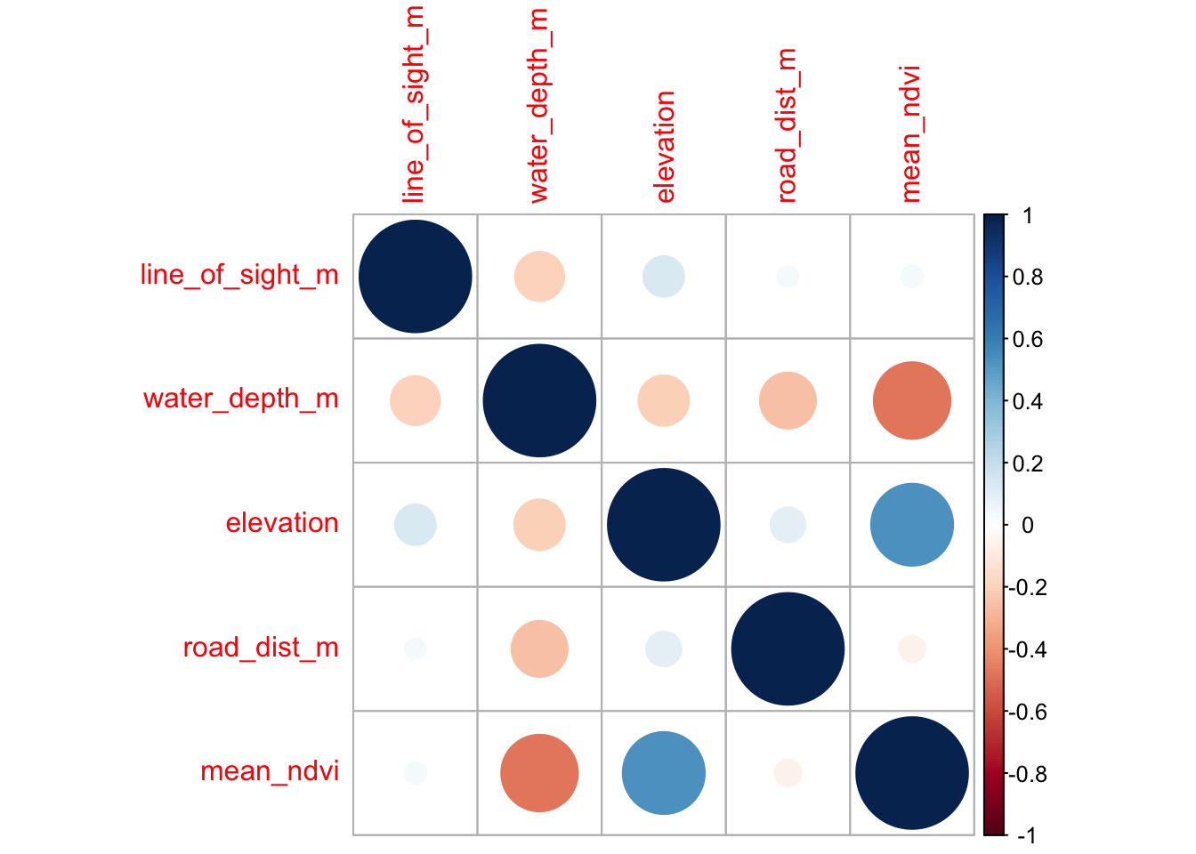
The cells denote pairwise correlations between the rows and the columns. The great thing about corrplot is customization option are near endless - see the corrplot vignette.

Let’s make a better, more informative, corrplot!

corrplot(M,                              #The correlation matrix we made
         method="color",                 # How we want the cells 
         type="upper",                   # Just show the upper part (it is usually mirrored)
         order="hclust",                 # Order the variables using the hclust method
         addCoef.col = "black",          # Add coefficient of correlation  
         tl.col="black", tl.srt=45,      # Control the text label color and rotation
         diag=F                          # Suppress the diagonal correlations (which are 1 anyway)
         )

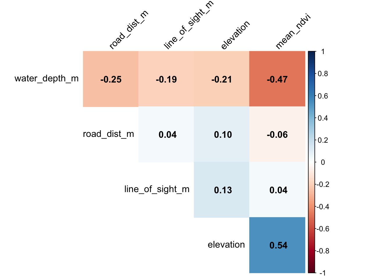
In general there is very low correlation between our different predictors! If we were seeing pairwise correlations >0.7 we perhaps wouldn’t include those in the same model.